

Video Intro to Bayesian Data Analysis, Part 3: How to do Bayes? This is the last video of a three part introduction to Bayesian data analysis aimed at you who isn’t necessarily that well-versed in probability theory but that do know a little bit of programming.
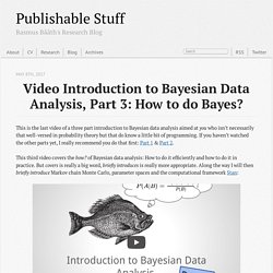
If you haven’t watched the other parts yet, I really recommend you do that first: Part 1 & Part 2. This third video covers the how? Of Bayesian data analysis: How to do it efficiently and how to do it in practice. But covers is really a big word, briefly introduces is really more appropriate. Along the way I will then briefly introduce Markov chain Monte Carlo, parameter spaces and the computational framework Stan: After having watched this video tutorial (and having done the exercises) you won’t be an expert in any way, like the expert fisherman depicted below by the master Hokusai.
How Bayesian inference works. Bayes’ theorem in three panels. In my last post, I walked through an intuition-building visualization I created to describe mixed-effects models for a nonspecialist audience.
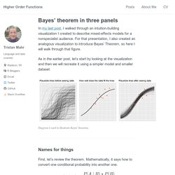
For that presentation, I also created an analogous visualization to introduce Bayes’ Theorem, so here I will walk through that figure. As in the earlier post, let’s start by looking at the visualization and then we will recreate it using a simpler model and smaller dataset. Names for things. What is a likelihood anyway? Fitting psychometric functions using STAN. Intro to Approximate Bayesian Computation (ABC) Many of the posts in this blog have been concerned with using MCMC based methods for Bayesian inference.
These methods are typically “exact” in the sense that they have the exact posterior distribution of interest as their target equilibrium distribution, but are obviously “approximate”, in that for any finite amount of computing time, we can only generate a finite sample of correlated realisations from a Markov chain that we hope is close to equilibrium. Approximate Bayesian Computation (ABC) methods go a step further, and generate samples from a distribution which is not the true posterior distribution of interest, but a distribution which is hoped to be close to the real posterior distribution of interest. Posteriors vs predictives. Bayesian Probability Is Not Subjective (It Only Seems Like It Is) Frequentists Are Closet Bayesians: Confidence Interval Edition. Illuminating a wide confidence interval Actually, all frequentists and Bayesians are logical probabilists, but if I put that in the title, few would believe it.

A man might call himself an Anti-Gravitational Theorist, a science which describes the belief that gravity is subject to human will. But the very moment that man takes a long walk off a short dock, he’s going to get wet. Musicians, drunks, and Oliver Cromwell. Bayes’ Theorem Using Trimmed Trees. Convenient and innocuous priors. Andrew Gelman has some interesting comments on non-informative priors this morning.

Rather than thinking of the prior as a static thing, think of it as a way to prime the pump. … a non-informative prior is a placeholder: you can use the non-informative prior to get the analysis started, then if your posterior distribution is less informative than you would like, or if it does not make sense, you can go back and add prior information. … At first this may sound like tweaking your analysis until you get the conclusion you want. A prior distribution cannot strictly be non-informative, but there are common intuitive notions of what it means to be non-informative.
Bayesian First Aid. So I have a secret project.

Come closer. I’m developing an R package that implements Bayesian alternatives to the most commonly used statistical tests. Yes you heard me, soon your t.testing days might be over! The package aims at being as easy as possible to pick up and use, especially if you are already used to the classical .test functions. The main gimmick is that the Bayesian alternatives will have the same calling semantics as the corresponding classical test functions save for the addition of bayes. to the beginning of the function name. The package does not aim at being some general framework for Bayesian inference or a comprehensive collection of Bayesian models. Short taxonomy of Bayes factors. January 21, 2014 Filed in: R | Statistics.
Writing a Metropolis-Hastings within Gibbs sampler in R for a 2PL IRT model. Last year, Brian Junker, Richard Patz, and I wrote an invited chapter for the (soon to be released) update of the classic text Handbook of Modern Item Response Theory (1996).

The chapter itself is meant to be an update of the classic IRT in MCMC papers Patz & Junker (1999a, 1999b). To support the chapter, I have put together an online supplement which gives a detailed walk-through of how to write a Metropolis-Hastings sampler for a simple psychometric model (in R, of course!). The table of contents is below: Stan - ShinyStan. Analysis & visualization GUI for MCMC ShinyStan provides visual and numerical summaries of model parameters and convergence diagnostics for MCMC simulations.

ShinyStan can be used to explore the output of any MCMC program (including but not limited to Stan, JAGS, BUGS, MCMCPack, NIMBLE, emcee, and SAS). Subjectivity in statistics. Understanding Naïve Bayes Classifier Using R. The Best Algorithms are the Simplest The field of data science has progressed from simple linear regression models to complex ensembling techniques but the most preferred models are still the simplest and most interpretable.
Among them are regression, logistic, trees and naive bayes techniques. Naive Bayes algorithm, in particular is a logic based technique which is simple yet so powerful that it is often known to outperform complex algorithms for very large datasets. Naive bayes is a common technique used in the field of medical science and is especially used for cancer detection. This article explains the underlying logic behind naive bayes algorithm and example implementation. How Probability defines Everything. Explaining Bayesian Networks through a football management problem. Today's Significance Magazine (the magazine of the Royal Statistical Society and the American Statistical Association) has published an article by Anthony Constantinou and Norman Fenton that explains, through the use of an example from football management, the kind of assumptions required to build useful Bayesian networks (BNs) for complex decision-making. The article highlights the need to fuse data with expert knowledge, and describes the challenges in doing so.
It also explains why, for fully optimised decision-making, extended versions of BNs, called Bayesian decision networks, are required. Intro to Greta. By Joseph Rickert I was surprised by greta. I had assumed that the tensorflow and reticulate packages would eventually enable R developers to look beyond deep learning applications and exploit the TensorFlow platform to create all manner of production-grade statistical applications.