

Constants and ARIMA models in R. This post is from my new book Forecasting: principles and practice, available freely online at OTexts.com/fpp/.
A non-seasonal ARIMA model can be written as or equivalently as where is the backshift operator, and is the mean of . Thus, the inclusion of a constant in a non-stationary ARIMA model is equivalent to inducing a polynomial trend of order. R Time Series Tutorial. The data sets used in this tutorial are available in astsa, the R package for the text.
A detailed tutorial (and more!) Is available in Appendix R of the text. This page is basically the quick fix from Edition 2 updated a bit. You can copy-and-paste the R commands (multiple lines are ok) from this page into R. Printed output is blue, and you wouldn't want to paste those lines into R, would you? This quick fix is meant for people who are just starting to use R for time series analysis. If you're new to R/Splus, I suggest reading R for Beginners (a pdf file) first. Functional and Parallel time series cross-validation. OMWP_2011_08.pdf. Forecasting time series using R - MelbourneRUG.pdf. Forecasting stock returns using ARIMA model with exogenous variable in R.
India has a lot to achieve in terms of becoming a developed nation from an economic standpoint.
An aspect which, in my opinion, is of utmost importance is the formation of structurally sound and robust financial markets. A prerequisite for that is active participation of educated and informed traders in the market place which would result in better price discovery and in turn better functioning market in general. Statistical modelling techniques supplemented with some subject understanding could be an informed trading strategy.
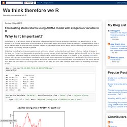
In the long run it might not be possible to outplay the market using a simple backward looking statistical model, but in the short run intelligent estimates based on model and subject matter expertise could prove to be helpful. In our previous posts with Infosys stock prices, we used basic visualization and simple linear regression techniques to try and predict the future returns from historical returns. Library(tseries, quietly = T) Forecasting: principles and practice. How does auto.arima() work ?
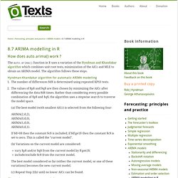
The auto.arima() function in R uses a variation of the Hyndman and Khandakar algorithm which combines unit root tests, minimization of the AICc and MLE to obtain an ARIMA model. The algorithm follows these steps. Hyndman-Khandakar algorithm for automatic ARIMA modelling The number of differences $d$ is determined using repeated KPSS tests.The values of $p$ and $q$ are then chosen by minimizing the AICc after differencing the data $d$ times. Rather than considering every possible combination of $p$ and $q$, the algorithm uses a stepwise search to traverse the model space. Choosing your own model. Time series cross-validation 2. Crete5.pdf. Welcome to a Little Book of R for Time Series! — Time Series 0.2 documentation. The ARIMAX model muddle. There is often confusion about how to include covariates in ARIMA models, and the presentation of the subject in various textbooks and in R help files has not helped the confusion.
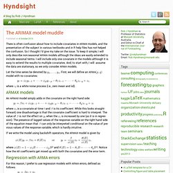
So I thought I’d give my take on the issue. To keep it simple, I will only describe non-seasonal ARIMA models although the ideas are easily extended to include seasonal terms. I will include only one covariate in the models although it is easy to extend the results to multiple covariates. And, to start with, I will assume the data are stationary, so we only consider ARMA models. Let the time series be denoted by . Model with no covariates: where is a white noise process (i.e., zero mean and iid). ARMAX models An ARMAX model simply adds in the covariate on the right hand side: is a covariate at time and. Functional and Parallel time series cross-validation. R Time Series Issues. ISSUE 1: When is the intercept the mean?
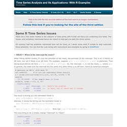
When fitting ARIMA models, R calls the estimate of the mean, the estimate of the intercept. This is ok if there's no AR term, but not if there is an AR term. For example, suppose x(t) = α + φ*x(t-1) + w(t) is stationary. Then taking expectations we have μ = α + φ*μ or α = μ*(1-φ). So, the intercept, α, is not the mean, μ, unless φ=0. . # generate an AR(1) with mean 50 set.seed(66) # so you can reproduce these results x = arima.sim(list(order=c(1,0,0), ar=.9), n=100) + 50 mean(x) [1] 50.60668 # the sample mean is close arima(x, order = c(1, 0, 0)) Coefficients: ar1 intercept <-- here's the problem 0.8971 50.6304 <-- or here, one of these has to change s.e. 0.0409 0.8365.
Time series - How to setup xreg argument in auto.arima() in R. R Time Series Tutorial.