
Cayley graph The Cayley graph of the free group on two generators a and b Definition[edit] Suppose that is a generating set. is a colored directed graph constructed as follows: [2] Each element of is assigned a vertex: the vertex set of is identified with Each generator of is assigned a color .For any the vertices corresponding to the elements and are joined by a directed edge of colour Thus the edge set consists of pairs of the form with providing the color. In geometric group theory, the set is usually assumed to be finite, symmetric (i.e. Examples[edit] Cayley graph of the dihedral group Dih4 on two generators a and b On two generators of Dih4, which are both self-inverse A Cayley graph of the dihedral group D4 on two generators a and b is depicted to the left. A different Cayley graph of Dih4 is shown on the right. b is still the horizontal reflection and represented by blue lines; c is a diagonal reflection and represented by green lines. Part of a Cayley graph of the Heisenberg group. . .
Libya's foreign minister flees to Britain - Africa Moussa Koussa, the Libyan foreign minister, has defected to the United Kingdom, the British foreign ministry has said. The ministry said in a statement that Koussa had arrived at Farnborough Airport, in the south of England, on a flight from Tunisia on Wednesday. "He travelled here under his own free will. He has told us that he is resigning his post. We are discussing this with him and we will release further details in due course," the statement said. "We encourage those around Gaddafi to abandon him and embrace a better future for Libya that allows political transition and real reform that meets the aspirations of the Libyan people." It added that Koussa was one of the most senior officials in Gaddafi's government with a role to represent it internationally, which is "something that he is no longer willing to do". Tunisia's TAP news agency said on Monday that Koussa had crossed over into Tunisia from Libya. "He is on a diplomatic mission," Mussa Ibrahim, the spokesman, said. Arms debate
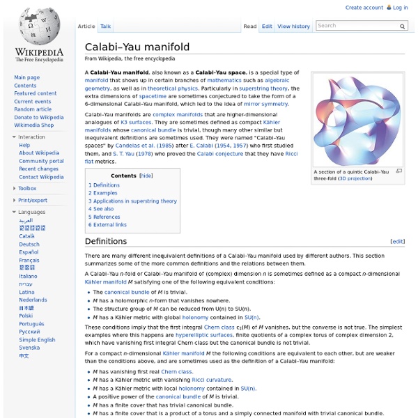
Hopf fibration The Hopf fibration can be visualized using a stereographic projection of S3 to R3 and then compressing R3 to a ball. This image shows points on S2 and their corresponding fibers with the same color. Pairwise linked keyrings mimic part of the Hopf fibration. In the mathematical field of topology, the Hopf fibration (also known as the Hopf bundle or Hopf map) describes a 3-sphere (a hypersphere in four-dimensional space) in terms of circles and an ordinary sphere. Discovered by Heinz Hopf in 1931, it is an influential early example of a fiber bundle. Technically, Hopf found a many-to-one continuous function (or "map") from the 3-sphere onto the 2-sphere such that each distinct point of the 2-sphere comes from a distinct circle of the 3-sphere (Hopf 1931). This fiber bundle structure is denoted meaning that the fiber space S1 (a circle) is embedded in the total space S3 (the 3-sphere), and p : S3 → S2 (Hopf's map) projects S3 onto the base space S2 (the ordinary 2-sphere).
grandma effect A study led by Prof Kristen Hawkes at the University of Utah provides new mathematical support for the ‘grandmother hypothesis,’ a theory that humans evolved longer adult lifespans than apes because grandmothers helped feed their grandchildren. Kristen Hawkes, a professor of anthropology with the University of Utah and co-author of the ‘grandmother hypothesis,’ a theory that humans evolved longer adult lifespans than apes because grandmothers helped feed their grandchildren (Lee J. Siegel / University of Utah) Prof Hawkes with colleagues proposed the hypothesis in 1997. It stemmed from observations by the scientists in the 80s when they lived with Hadza hunter-gatherer people in Tanzania and watched older women spend their days collecting tubers and other foods for their grandchildren. “Grandmothering was the initial step toward making us who we are,” said Prof Hawkes, who co-authored the study published in the Proceedings of the Royal Society B. Bibliographic information: Peter S.
Poincaré disk model Metric[edit] If u and v are two vectors in real n-dimensional vector space Rn with the usual Euclidean norm, both of which have norm less than 1, then we may define an isometric invariant by where denotes the usual Euclidean norm. Such a distance function is defined for any two vectors of norm less than one, and makes the set of such vectors into a metric space which is a model of hyperbolic space of constant curvature −1. The associated metric tensor of the Poincaré disk model is given by where the xi are the Cartesian coordinates of the ambient Euclidean space. Relation to the hyperboloid model[edit] The hyperboloid model can be seen as the equation of t2=x2+y2+1 can can be used to construct a Poincaré disk model as a perspective projection viewed from (t=-1,x=0,y=0), projecting the upper half hyperboloid onto an (x,y) unit disk at t=0. The Poincaré disk model, as well as the Klein model, are related to the hyperboloid model projectively. Angles[edit] Artistic realizations[edit] M.
ocean Permy? Convergence of Fourier series Determination of convergence requires the comprehension of pointwise convergence, uniform convergence, absolute convergence, Lp spaces, summability methods and the Cesàro mean. Preliminaries[edit] Consider ƒ an integrable function on the interval [0,2π]. are defined by the formula It is common to describe the connection between ƒ and its Fourier series by The notation ~ here means that the sum represents the function in some sense. The question we will be interested in is: Do the functions (which are functions of the variable t we omitted in the notation) converge to ƒ and in which sense? Before continuing the Dirichlet kernel needs to be introduced. , inserting it into the formula for and doing some algebra will give that where ∗ stands for the periodic convolution and is the Dirichlet kernel which has an explicit formula, The Dirichlet kernel is not a positive kernel, and in fact, its norm diverges, namely a fact that will play a crucial role in the discussion. If for and and therefore, if Suppose
Open Source Ecology Schwarz triangle In geometry, a Schwarz triangle, named after Hermann Schwarz, is a spherical triangle that can be used to tile a sphere, possibly overlapping, through reflections in its edges. They were classified in (Schwarz 1873). These can be defined more generally as tessellations of the sphere, the Euclidean plane, or the hyperbolic plane. Each Schwarz triangle on a sphere defines a finite group, while on the Euclidean or hyperbolic plane they define an infinite group. A Schwarz triangle is represented by three rational numbers (p q r) each representing the angle at a vertex. The value n/d means the vertex angle is d/n of the half-circle. "2" means a right triangle. Solution space[edit] A fundamental domain triangle, (p q r), can exist in different space depending on this constraint: Graphical representation[edit] A Schwarz triangle is represented graphically by a triangular graph. Order-2 edges represent perpendicular mirrors that can be ignored in this diagram. A list of Schwarz triangles[edit]
truthdig Humans must immediately implement a series of radical measures to halt carbon emissions or prepare for the collapse of entire ecosystems and the displacement, suffering and death of hundreds of millions of the globe’s inhabitants, according to a report commissioned by the World Bank. The continued failure to respond aggressively to climate change, the report warns, will mean that the planet will inevitably warm by at least 4 degrees Celsius (7.2 degrees Fahrenheit) by the end of the century, ushering in an apocalypse. The 84-page document,“Turn Down the Heat: Why a 4°C Warmer World Must Be Avoided,” was written for the World Bank by the Potsdam Institute for Climate Impact Research and Climate Analytics and published last week. The picture it paints of a world convulsed by rising temperatures is a mixture of mass chaos, systems collapse and medical suffering like that of the worst of the Black Plague, which in the 14th century killed 30 to 60 percent of Europe’s population.
Point groups in three dimensions In geometry, a point group in three dimensions is an isometry group in three dimensions that leaves the origin fixed, or correspondingly, an isometry group of a sphere. It is a subgroup of the orthogonal group O(3), the group of all isometries that leave the origin fixed, or correspondingly, the group of orthogonal matrices. O(3) itself is a subgroup of the Euclidean group E(3) of all isometries. Symmetry groups of objects are isometry groups. The point groups in three dimensions are heavily used in chemistry, especially to describe the symmetries of a molecule and of molecular orbitals forming covalent bonds, and in this context they are also called molecular point groups. Finite Coxeter groups are a special set of point groups generated purely by a set of reflectional mirrors passing through the same point. Group structure[edit] O(3) is the direct product of SO(3) and the group generated by inversion (denoted by its matrix −I): where isometry ( A, I ) is identified with A.
polit Conservationist Villarceau circles Conceptual animation showing how a slant cut torus reveals a pair of circles, known as Villarceau circles In geometry, Villarceau circles /viːlɑrˈsoʊ/ are a pair of circles produced by cutting a torus diagonally through the center at the correct angle. Given an arbitrary point on a torus, four circles can be drawn through it. Example[edit] For example, let the torus be given implicitly as the set of points on circles of radius three around points on a circle of radius five in the xy plane Slicing with the z = 0 plane produces two concentric circles, x2 + y2 = 22 and x2 + y2 = 82. Two example Villarceau circles can be produced by slicing with the plane 3x = 4z. and The slicing plane is chosen to be tangent to the torus while passing through its center. Existence and equations[edit] A proof of the circles’ existence can be constructed from the fact that the slicing plane is tangent to the torus at two points. The cross-section of the swept surface in the xz plane now includes a second circle.
Hadamard space In an Hadamard space, a triangle is hyperbolic; that is, the middle one in the picture. In fact, any complete metric space where a triangle is hyperbolic is an Hadamard space. In geometry, an Hadamard space, named after Jacques Hadamard, is a non-linear generalization of a Hilbert space. The point m is then the midpoint of x and y: In a Hilbert space, the above inequality is equality (with ), and in general an Hadamard space is said to be flat if the above inequality is equality. fixes the circumcenter of B. The basic result for a non-positively curved manifold is the Cartan–Hadamard theorem. See also[edit] References[edit] Jump up ^ The assumption on "nonempty" has meaning: a fixed point theorem often states the set of fixed point is an Hadamard space.