
Kernel Methods for Pattern Analysis - The Book Connectionism Connectionism is a set of approaches in the fields of artificial intelligence, cognitive psychology, cognitive science, neuroscience, and philosophy of mind, that models mental or behavioral phenomena as the emergent processes of interconnected networks of simple units. There are many forms of connectionism, but the most common forms use neural network models. Basic principles[edit] The central connectionist principle is that mental phenomena can be described by interconnected networks of simple and often uniform units. The form of the connections and the units can vary from model to model. For example, units in the network could represent neurons and the connections could represent synapses. Spreading activation[edit] In most connectionist models, networks change over time. Neural networks[edit] Most of the variety among neural network models comes from: Biological realism[edit] Learning[edit] The weights in a neural network are adjusted according to some learning rule or algorithm.
Perceptron Een perceptron (of meerlaags perceptron) is een neuraal netwerk waarin de neuronen in verschillende lagen met elkaar verbonden zijn. Een eerste laag bestaat uit ingangsneuronen, waar de inputsignalen aangelegd worden. Vervolgens zijn er één of meerdere 'verborgen’ lagen, die zorgen voor meer 'intelligentie' en ten slotte is er de uitgangslaag, die het resultaat van het perceptron weergeeft. Alle neuronen van een bepaalde laag zijn verbonden met alle neuronen van de volgende laag, zodat het ingangssignaal voort propageert door de verschillende lagen heen. Single-layer Perceptron[bewerken] De single-layer perceptron is de simpelste vorm van een neuraal netwerk, in 1958 door Rosenblatt ontworpen (ook wel Rosenblatt's perceptron genoemd). Rosenblatt's Perceptron Het is mogelijk het aantal klassen uit te breiden naar meer dan twee, wanneer de output layer wordt uitgebreid met meerdere output neurons. Trainingsalgoritme[bewerken] Begrippen: = inputvector = gewichtsvector (weights vector) Met = bias
Autoencoder An autoencoder, autoassociator or Diabolo network[1]:19 is an artificial neural network used for learning efficient codings.[2] The aim of an auto-encoder is to learn a compressed, distributed representation (encoding) for a set of data, typically for the purpose of dimensionality reduction. Overview[edit] Architecturally, the simplest form of the autoencoder is a feedforward, non-recurrent neural net that is very similar to the multilayer perceptron (MLP), with an input layer, an output layer and one or more hidden layers connecting them. The difference with the MLP is that in an autoencoder, the output layer has equally many nodes as the input layer, and instead of training it to predict some target value y given inputs x, an autoencoder is trained to reconstruct its own inputs x. I.e., the training algorithm can be summarized as For each input x, Do a feed-forward pass to compute activations at all hidden layers, then at the output layer to obtain an output x̂ Training[edit]
Feedforward neural network In a feed forward network information always moves one direction; it never goes backwards. A feedforward neural network is an artificial neural network where connections between the units do not form a directed cycle. This is different from recurrent neural networks. The feedforward neural network was the first and simplest type of artificial neural network devised. In this network, the information moves in only one direction, forward, from the input nodes, through the hidden nodes (if any) and to the output nodes. Single-layer perceptron[edit] The simplest kind of neural network is a single-layer perceptron network, which consists of a single layer of output nodes; the inputs are fed directly to the outputs via a series of weights. A perceptron can be created using any values for the activated and deactivated states as long as the threshold value lies between the two. Perceptrons can be trained by a simple learning algorithm that is usually called the delta rule. (times See also[edit]
Feature learning Feature learning or representation learning[1] is a set of techniques in machine learning that learn a transformation of "raw" inputs to a representation that can be effectively exploited in a supervised learning task such as classification. Feature learning algorithms themselves may be either unsupervised or supervised, and include autoencoders,[2] dictionary learning, matrix factorization,[3] restricted Boltzmann machines[2] and various form of clustering.[2][4][5] When the feature learning can be performed in an unsupervised way, it enables a form of semisupervised learning where first, features are learned from an unlabeled dataset, which are then employed to improve performance in a supervised setting with labeled data.[6][7] Clustering as feature learning[edit] K-means clustering can be used for feature learning, by clustering an unlabeled set to produce k centroids, then using these centroids to produce k additional features for a subsequent supervised learning task. See also[edit]
Protein Secondary Structure Prediction with Neural Nets: Feed-Forward Networks Introduction to feed-forward nets Feed-forward nets are the most well-known and widely-used class of neural network. The popularity of feed-forward networks derives from the fact that they have been applied successfully to a wide range of information processing tasks in such diverse fields as speech recognition, financial prediction, image compression, medical diagnosis and protein structure prediction; new applications are being discovered all the time. (For a useful survey of practical applications for feed-forward networks, see [Lisboa, 1992].) In common with all neural networks, feed-forward networks are trained, rather than programmed, to carry out the chosen information processing tasks. The feed-forward architecture Feed-forward networks have a characteristic layered architecture, with each layer comprising one or more simple processing units called artificial neurons or nodes. Diagram of 2-Layer Perceptron Training a feed-forward net 1. 2. 3.
Multilayer perceptron A multilayer perceptron (MLP) is a feedforward artificial neural network model that maps sets of input data onto a set of appropriate outputs. A MLP consists of multiple layers of nodes in a directed graph, with each layer fully connected to the next one. Except for the input nodes, each node is a neuron (or processing element) with a nonlinear activation function. MLP utilizes a supervised learning technique called backpropagation for training the network.[1][2] MLP is a modification of the standard linear perceptron and can distinguish data that are not linearly separable.[3] Theory[edit] Activation function[edit] If a multilayer perceptron has a linear activation function in all neurons, that is, a linear function that maps the weighted inputs to the output of each neuron, then it is easily proved with linear algebra that any number of layers can be reduced to the standard two-layer input-output model (see perceptron). is the output of the th node (neuron) and Layers[edit] in the , where
Self-organizing map A self-organizing map (SOM) or self-organizing feature map (SOFM) is a type of artificial neural network (ANN) that is trained using unsupervised learning to produce a low-dimensional (typically two-dimensional), discretized representation of the input space of the training samples, called a map. Self-organizing maps are different from other artificial neural networks in the sense that they use a neighborhood function to preserve the topological properties of the input space. This makes SOMs useful for visualizing low-dimensional views of high-dimensional data, akin to multidimensional scaling. The model was first described as an artificial neural network by the Finnish professor Teuvo Kohonen, and is sometimes called a Kohonen map or network.[1][2] Like most artificial neural networks, SOMs operate in two modes: training and mapping. A self-organizing map consists of components called nodes or neurons. Large SOMs display emergent properties. Learning algorithm[edit] Variables[edit]
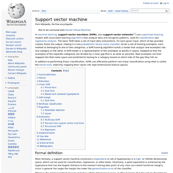
Restricted Boltzmann machine Diagram of a restricted Boltzmann machine with three visible units and four hidden units (no bias units). A restricted Boltzmann machine (RBM) is a generative stochastic neural network that can learn a probability distribution over its set of inputs. RBMs were initially invented under the name Harmonium by Paul Smolensky in 1986,[1] but only rose to prominence after Geoffrey Hinton and collaborators invented fast learning algorithms for them in the mid-2000s. RBMs have found applications in dimensionality reduction,[2] classification,[3] collaborative filtering, feature learning[4] and topic modelling.[5] They can be trained in either supervised or unsupervised ways, depending on the task. Restricted Boltzmann machines can also be used in deep learning networks. In particular, deep belief networks can be formed by "stacking" RBMs and optionally fine-tuning the resulting deep network with gradient descent and backpropagation.[7] Structure[edit] and visible unit for the visible units and where
History of the Perceptron History of the Perceptron The evolution of the artificial neuron has progressed through several stages. The roots of which, are firmly grounded within neurological work done primarily by Santiago Ramon y Cajal and Sir Charles Scott Sherrington . Working from the beginnings of neuroscience, Warren McCulloch and Walter Pitts in their 1943 paper, "A Logical Calculus of Ideas Immanent in Nervous Activity," contended that neurons with a binary threshold activation function were analogous to first order logic sentences. The McCulloch-Pitts neuron worked by inputting either a 1 or 0 for each of the inputs, where 1 represented true and 0 false. This table shows the basic “and” function such that, if x1 and x2 are both false, then the output of combining these two will also be false. This follows also for the “or” function, if we switch the threshold value to 1. One of the difficulties with the McCulloch-Pitts neuron was its simplicity. The activation function then becomes: x = f(b)
Online machine learning Online machine learning is used in the case where the data becomes available in a sequential fashion, in order to determine a mapping from the dataset to the corresponding labels. The key difference between online learning and batch learning (or "offline" learning) techniques, is that in online learning the mapping is updated after the arrival of every new datapoint in a scalable fashion, whereas batch techniques are used when one has access to the entire training dataset at once. Online learning could be used in the case of a process occurring in time, for example the value of a stock given its history and other external factors, in which case the mapping updates as time goes on and we get more and more samples. Ideally in online learning, the memory needed to store the function remains constant even with added datapoints, since the solution computed at one step is updated when a new datapoint becomes available, after which that datapoint can then be discarded. , where on . , such that .
Dimensionality reduction In machine learning and statistics, dimensionality reduction or dimension reduction is the process of reducing the number of random variables under consideration,[1] and can be divided into feature selection and feature extraction.[2] Feature selection[edit] Feature extraction[edit] The main linear technique for dimensionality reduction, principal component analysis, performs a linear mapping of the data to a lower-dimensional space in such a way that the variance of the data in the low-dimensional representation is maximized. Principal component analysis can be employed in a nonlinear way by means of the kernel trick. An alternative approach to neighborhood preservation is through the minimization of a cost function that measures differences between distances in the input and output spaces. Dimension reduction[edit] See also[edit] Notes[edit] Jump up ^ Roweis, S. References[edit] Fodor,I. (2002) "A survey of dimension reduction techniques". External links[edit]
Artificial neural network An artificial neural network is an interconnected group of nodes, akin to the vast network of neurons in a brain. Here, each circular node represents an artificial neuron and an arrow represents a connection from the output of one neuron to the input of another. For example, a neural network for handwriting recognition is defined by a set of input neurons which may be activated by the pixels of an input image. After being weighted and transformed by a function (determined by the network's designer), the activations of these neurons are then passed on to other neurons. This process is repeated until finally, an output neuron is activated. This determines which character was read. Like other machine learning methods - systems that learn from data - neural networks have been used to solve a wide variety of tasks that are hard to solve using ordinary rule-based programming, including computer vision and speech recognition. Background[edit] History[edit] Farley and Wesley A. Models[edit] or both