

Rhinoceros - NURBS. NURBS, Non-Uniform Rational B-Splines, are mathematical representations of 3‑D geometry that can accurately describe any shape from a simple 2‑D line, circle, arc, or curve to the most complex 3‑D organic free-form surface or solid.
Because of their flexibility and accuracy, NURBS models can be used in any process from illustration and animation to manufacturing. NURBS geometry has five important qualities that make it an ideal choice for computer-aided modeling. Several industry‑standard methods are used to exchange NURBS geometry. This means that customers are able to move their valuable geometric models between various modeling, rendering, animation, and engineering analysis programs. They can store geometric information in a way that will be usable for the foreseeable future. NURBS curves and surfaces behave in similar ways and share terminology. Degree The degree is a positive whole number. (18) Computing a tangent plane. Overview (JTS Topology Suite 1.15.0-SNAPSHOT API) Python & OpenGL for Scientific Visualization.
For the really impatient, you can try to run the code in the teaser image above.

If this works, a window should open on your desktop with a red color in the background. If you now want to understand how this works, you'll have to read the text below. Preliminaries The main difficulty for newcomers in programming modern OpenGL is that it requires to understand a lot of different concepts at once and then, to perform a lot of operations before rendering anything on screen.
This complexity implies that there are many places where your code can be wrong, both at the conceptual and code level. Normalize Device Coordinates Figure. Meshmash/Plankton: A C# half-edge mesh data structure, and components for using this in Grasshopper/Rhino. Cocoon – bespoke geometry. Cocoon is an add-on to McNeel’s Grasshopper visual scripting interface for Rhinoceros.
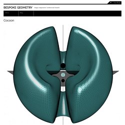
Cocoon is a fairly straightforward implementation of the Marching Cubes algorithm for turning iso-surfaces into polygonal meshes. It is geared specifically toward wrapping existing geometric elements, and works with combinations of points, breps and curves, allowing users to vary a number of parameters that enhance sculptural potentials. It is still rough (and there are definitely a number of other approaches to level sets and isosurfacing that are faster, more robust, more elegant, and/or have more potential) but due to time constraints related to other work I am doing – now and into the near future – I thought it effective and fun enough that it was worth it to make this available to the community.
As such, though, general caveats apply: it’s probably easy to break, and it will definitely generate some artifacts. Aether – simple speedy spatial fields for Grasshopper - Grasshopper. Marching Cubes: Curve Wrapping & More Metaballs - Grasshopper. UPDATE: 30-Jan-2014. Implicit surfaces. Also known as "Metaballs", "Blobbies", "Soft objects" Written by Paul Bourke June 1997 Introduction Most computer based 3D geometric modelling is done with basic primitives such as lines, planes, boxes, etc.
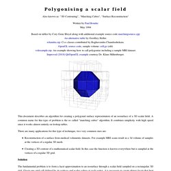
Many smooth and deformable objects are difficult or inefficient to represent with such building blocks, even if primitives such as spheres or Bezier/spline surfaces are used. An increasingly popular approach has been the use of field functions in 3D, the surfaces being isosurfaces through the field. The following summarises three common methods for creating so called "implicit surfaces". Polygonising a scalar field (Marching Cubes) Also known as: "3D Contouring", "Marching Cubes", "Surface Reconstruction" Written by Paul Bourke May 1994 Based on tables by Cory Gene Bloyd along with additional example source code marchingsource.cppAn alternative table by Geoffrey Heller.rchandra.zip: C++ classes contributed by Raghavendra Chandrashekara.OpenGL source code, sample volume: cell.gz (old)volexample.zip: An example showing how to call polygonise including a sample MRI dataset.Improved (2018) Qt/OpenGL example courtesy Dr.
Klaus Miltenberger. Isosurface. An isosurface is a three-dimensional analog of an isoline.
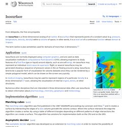
It is a surface that represents points of a constant value (e.g. pressure, temperature, velocity, density) within a volume of space; in other words, it is a level set of a continuous function whose domain is 3D-space. Isosurface of vorticity trailed from a propeller blade. Note that this is an isosurface plotted with a colormapped slice. Applications[edit] Isosurfaces are normally displayed using computer graphics, and are used as data visualization methods in computational fluid dynamics (CFD), allowing engineers to study features of a fluid flow (gas or liquid) around objects, such as aircraft wings. Numerous other disciplines that are interested in three-dimensional data often use isosurfaces to obtain information about pharmacology, chemistry, geophysics and meteorology. Implementation Algorithms[edit]
K3DSurf : 3d surface generator. Advances in Architectural Geometry 2016-eBook. Geometry and Physics. A Short Course in Computational Geometry and Topology (SpringerBriefs in Applied Sciences and Technology): Herbert Edelsbrunner: 9783319059563: Amazon.com: Books. Handbook of Discrete and Computational Geometry - 3rd edition.
Applied Geometry. Applied Geometry. Education Professional Experience Research assistant, Institute of Discrete Mathematics and Geometry, TU Wien, since 02/2011 FWF Project assistant, Project Applications of Higher Geometries (PI: H.
Pottmann), 05/2010 - 01/2011 Research assistant, Institute of Geometry, TU Graz, 03/2007 - 04/2010. A-Star (A*) Implementation in C# (Path Finding, PathFinder) WEBINAR: On-demand webcast How to Boost Database Development Productivity on Linux, Docker, and Kubernetes with Microsoft SQL Server 2017 REGISTER > Introduction.

Shortest Path. [GHX: 0.8.0066] This is the continuation of my scripting experiment within Grasshopper.
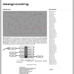
Like minimum spanning tree algorithm, this is also a famous problem of computational geometry. I’m now coding faster and understanding the namespace easier in Grasshopper. This time, challenge was to implement Dijkstra’s algorithm of shortest paths. Dijkstra's algorithm. The algorithm exists in many variants; Dijkstra's original variant found the shortest path between two nodes,[3] but a more common variant fixes a single node as the "source" node and finds shortest paths from the source to all other nodes in the graph, producing a shortest-path tree.
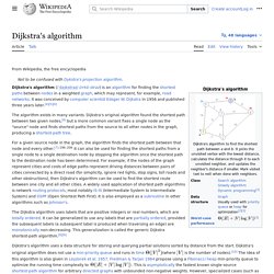
For a given source node in the graph, the algorithm finds the shortest path between that node and every other.[4]:196–206 It can also be used for finding the shortest paths from a single node to a single destination node by stopping the algorithm once the shortest path to the destination node has been determined. For example, if the nodes of the graph represent cities and edge path costs represent driving distances between pairs of cities connected by a direct road, Dijkstra's algorithm can be used to find the shortest route between one city and all other cities.