

Likelihood Ratio Test in R with Example » finnstats. Simple Linear Regression in r » Guide » finnstats. Moving Away From R². The perils of using it and how to… In this example, we are going to create some data.
What we want to do is define what our signal is going to be, introduce varying levels of noise, and see how R² reacts. Our signal: The true coefficient of X being equal to 1.2 The noise: Random addition of numbers with a mean of 0 and increasing standard deviation. To accomplish this we are going to use the following code to generate data. x1 <- seq(1,10,length.out = 500) y1 <- 2 + 1.2*x1 + rnorm(500,0,sd = 1) For x1 the computer is going to generate 500 numbers between 1 and 10. We will create 4 graphs and linear regressions to see how our results change with increasing standard deviation. If R² measures our signal or the strength of it, it should stay roughly equal.
Testing The Equality of Regression Coefficients. You have two predictors in your model.

One seems to have a stronger coefficient than the other. But is it significant? Example: when predicting a worker’s salary, is the standardized coefficient of number of extra hours (xtra_hours) really larger than that of number of compliments given the to boss n_comps? Library(parameters) library(effectsize) data("hardlyworking", package = "effectsize") hardlyworkingZ <- standardize(hardlyworking) m <- lm(salary ~ xtra_hours + n_comps, data = hardlyworkingZ) model_parameters(m) Here are 4 methods to test coefficient equality in R. Notes - If we were interested in the unstandardized coefficient, we would not need to first standardize the data. - Note that if one parameter was positive, and the other was negative, one of the terms would need to be first reversed (-X) to make this work. Method 1: As Model Comparisons Based on this awesome tweet.
Rolling Regression and Pairs Trading in R – Predictive Hacks. In a previous post, we have provided an example of Rolling Regression in Python to get the market beta coefficient.
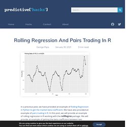
We have also provided an example of pairs trading in R. In this post, we will provide an example of rolling regression in R working with the rollRegres package. We will provide an example of getting the beta coefficient between two co-integrated stocks in a rolling window of n observations. What is a Rolling Regression The rolling regression is simply a dynamic regression within a rolling moving window.
Correlation Analysis in R, Part 1: Basic Theory – Data Enthusiast's Blog. Introduction There are probably tutorials and posts on all aspects of correlation analysis, including on how to do it in R.
So why more? How to Perform Feature Selection for Regression Data. Feature selection is the process of identifying and selecting a subset of input variables that are most relevant to the target variable.
Perhaps the simplest case of feature selection is the case where there are numerical input variables and a numerical target for regression predictive modeling. This is because the strength of the relationship between each input variable and the target can be calculated, called correlation, and compared relative to each other. LmSubsets: Exact variable-subset selection in linear regression. The R package lmSubsets for flexible and fast exact variable-subset selection is introduced and illustrated in a weather forecasting case study.
Citation Hofmann M, Gatu C, Kontoghiorghes EJ, Colubi A, Zeileis A (2020). What is Multicollinearity? Here's Everything You Need to Know - Analytics Vidhya. Untitled. Untitled. This article will be copy edited and may be changed before publication.
The R Package trafo for Transforming Linear Regression Models Lily Medina, Ann-Kristin Kreutzmann, Natalia Rojas-Perilla and Piedad Castro Abstract Researchers and data-analysts often use the linear regression model for descriptive, predictive, and inferential purposes. This model relies on a set of assumptions that, when not satisfied, yields biased results and noisy estimates. A common problem that can be solved in many ways – use of less restrictive methods (e.g. generalized linear regression models or non-parametric methods ), variance corrections or transformations of the response variable just to name a few.
Propensity Score Matching in R. Regression analysis is one of the most requested machine learning methods in 2019.
One group of regression analysis for measuring effects and to evaluate the statistical effect of covariates is Propensity Score Matching (PSM). This method is well suited to investigate if the covariates are changing the effects of the estimates in the regression model. It can, therefore, be used to design the regression model to be more accurate and efficient. Cvms 0.1.0 released on CRAN. After a fairly long life on GitHub, my R package, cvms, for cross-validating linear and logistic regression, is finally on CRAN!
With a few additions in the past months, this is a good time to catch you all up on the included functionality. For examples, check out the readme on GitHub! The main purpose of cvms is to allow researchers to quickly compare their models with cross-validation, with a tidy output containing the relevant metrics. Linear Regression · UC Business Analytics R Programming Guide. Introducing olsrr - Rsquared Academy Blog. I am pleased to announce the olsrr package, a set of tools for improved output from linear regression models, designed keeping in mind beginner/intermediate R users.
The package includes: comprehensive regression outputvariable selection proceduresheteroskedasticiy, collinearity diagnostics and measures of influencevarious plots and underlying data If you know how to build models using lm(), you will find olsrr very useful. Most of the functions use an object of class lm as input. So you just need to build a model using lm() and then pass it onto the functions in olsrr. Installation install.packages("olsrr") devtools::install_github("rsquaredacademy/olsrr") Shiny App olsrr includes a shiny app which can be launched using ols_launch_app() or try the live version here. Combining automatically factor levels in R. Each time we face real applications in an applied econometrics course, we have to deal with categorial variables.
And the same question arise, from students : how can we combine automatically factor levels ? Is there a simple R function ? I did upload a few blog posts, over the pas years. But so far, nothing satistfying. Let me write down a few lines about what could be done. N=200 set.seed(1) x1=runif(n) x2=runif(n) y=1+2*x1-x2+rnorm(n,0,.2) LB=sample(LETTERS[1:10]) b=data.frame(y=y,x1=x1, x2=cut(x2,breaks= c(-1,.05,.1,.2,.35,.4,.55,.65,.8,.9,2), labels=LB)) str(b) 'data.frame': 200 obs. of 3 variables: $ y : num 1.345 1.863 1.946 2.481 0.765 ... $ x1: num 0.266 0.372 0.573 0.908 0.202 ... $ x2: Factor w/ 10 levels "I","A","H","F",..: 4 4 6 4 3 6 7 3 4 8 ... table(b$x2)[LETTERS[1:10]] A B C D E F G H I J 11 12 23 34 23 36 12 32 3 14 There is one (continuous) dependent variable y, one continuous covariable x1 and one categorical variable x2, with here ten levels.
15 Types of Regression you should know. Regression techniques are one of the most popular statistical techniques used for predictive modeling and data mining tasks. On average, analytics professionals know only 2-3 types of regression which are commonly used in real world. They are linear and logistic regression. But the fact is there are more than 10 types of regression algorithms designed for various types of analysis. BreakDown plots for the linear model. Przemyslaw Biecek Here we will use the wine quality data ( to present the breakDown package for lm models. First, let’s download the data from URL. Data R Value: Machine Learning. Linear Regression Full Example (Boston Housing). It is important to mention that the present posts began as a personal way of practicing R programming and machine learning. Subsequently feedback from the community, urged me to continue performing these exercises and sharing them. The bibliography and corresponding authors are cited at all times and it is a way of honoring them and giving them the credit they deserve for their work.
Regtools. Let’s take a look at the data set prgeng, some Census data for California engineers and programmers in the year 2000. The response variable in this example is wage income, and the predictors are age, number of weeks worked, and dummy variables for MS and PhD degrees. (Some data wrangling was performed first; type ? Knnest for the details.) The fit assessment techniques in regtools gauge the fit of parametric models by comparing to nonparametric ones. Since the latter are free of model bias, they are very useful in assessing the parametric models. The function nonparvsxplot() plots the nonparametric fits against each predictor variable, for instance to explore nonlinear effects. Of course, the effects of the other predictors don’t show up here, but there does seem to be a quadratic effect. So, after fitting the linear model, run parvsnonparplot(), which plots the fit of the parametric model against the nonparametric one.
Going Deeper into Regression Analysis with Assumptions, Plots & Solutions. First steps with Non-Linear Regression in R. Using segmented regression to analyse world record running times. By Andrie de Vries. Applied Statistical Theory: Quantile Regression. This is part two of the ‘applied statistical theory’ series that will cover the bare essentials of various statistical techniques. As analysts, we need to know enough about what we’re doing to be dangerous and explain approaches to others. It’s not enough to say “I used X because the misclassification rate was low.”
Standard linear regression summarizes the average relationship between a set of predictors and the response variable. represents the change in the mean value of. A function to help graphical model checks of lm and ANOVA. Using and interpreting different contrasts in linear models in R. When building a regression model with categorical variables with more than two levels (ie “Cold”, “Freezing”, “Warm”) R is doing internally some transformation to be able to compute regression coefficient.
R Tutorial Series: Graphic Analysis of Regression Assumptions. Linear Models. Notes on chapter 3 of Introduction to Statistical Learning and the Stanford Online Statistical Learning class. Testing the assumptions of linear regression. Quantitative models always rest on assumptions about the way the world works, and regression models are no exception. R tips pages. Regression on categorical variables. Model Validation: Interpreting Residual Plots.
GLM – Evaluating Logistic Regression Models (part 3) Continuous piecewise linear regression. Visualization in regression analysis. Binary classif. eval. in R via ROCR.